Compression of floating point timeseries
I recently had cause to investigate fast methods of storing and transferring financial timeseries. Naively, timeseries can be represented in memory or on disk as simple dense arrays of floating point numbers. This is an attractive representation with many nice properties:
- Straightforward and widely used.
- You have random access to the nth element of the timeseries with no further indexes required.
- Excellent locality-of-reference for applications that process timeseries in time order, which is the common case.
- Often natively supported by CPU vector instructions.
However, it is not a particularly space-efficient representation. Financial timeseries have considerable structure (e.g. Vodafone’s price on T is likely to be very close to the price on T+1), and this structure can be exploited by compression algorithms to greatly reduce storage requirements. This is important either when you need to store a large number of timeseries, or need to transfer a smaller number of timeseries over a bandwidth-constrained network link.
Timeseries compression has recieved quite a bit of attention from both the academic/scientific programming community (see e.g. FPC and PFOR) and also practicioner communities such as the demoscene (see this presentation by a member of Farbrausch). This post summarises my findings about the effect that a number of easy-to-implement “filters” have on the final compression ratio.
In the context of compression algorithms, filters are simple invertible transformations that are applied to the stream in the hopes of making the stream more compressible by subsequent compressors. Perhaps the canonical example of a filter is the Burrows-Wheeler transform, which has the effect of moving runs of similar letters together. Some filters will turn a decompressed input stream (from the user) of length N into an output stream (fed to the compressor) of length N, but in general filters will actually have the effect of making the stream longer. The hope is that the gains to compressability are enough to recover the bytes lost to any encoding overhead imposed by the filter.
In my application, I was using the compression as part of an RPC protocol that would be used interactively, so I wanted keep decompression time very low, and for ease-of-deployment I wanted to get results in the context of Java without making use of any native code. Consequently I was interested in which choice of filter and compression algorithm would give a good tradeoff between performance and compression ratio.
I determined this experimentally. In my experiments, I used timeseries associated with 100 very liquid US stocks retrieved from Yahoo Finance, amounting to 69MB of CSVs split across 6 fields per stock (open/high/low/close and adjusted close prices, plus volume). This amounted to 12.9 million floating point numbers.
Choice of compressor
To decide which compressors were contenders, I compressed these price timeseries with a few pure-Java implementations of the algorithms:
| Compressor | Compression time (s) | Decompression time (s) | Compression ratio |
|---|---|---|---|
| None | 0.0708 | 0.0637 | 1.000 |
| Snappy (org.iq80.snappy:snappy-0.3) | 0.187 | 0.115 | 0.843 |
| Deflate BEST_SPEED (JDK 8) | 4.59 | 4.27 | 0.602 |
| Deflate DEFAULT_COMPRESSION (JDK 8) | 5.46 | 4.29 | 0.582 |
| Deflate BEST_COMPRESSION (JDK 8) | 7.33 | 4.28 | 0.580 |
| BZip2 MIN_BLOCKSIZE (org.apache.commons:commons-compress-1.10) | 1.79 | 0.756 | 0.540 |
| BZip2 MAX_BLOCKSIZE (org.apache.commons:commons-compress-1.10) | 1.73 | 0.870 | 0.515 |
| XZ PRESET_MIN (org.apache.commons:commons-compress-1.10 + org.tukaani:xz-1.5) | 2.66 | 1.20 | 0.469 |
| XZ PRESET_DEFAULT (org.apache.commons:commons-compress-1.10 + org.tukaani:xz-1.5) | 9.56 | 1.15 | 0.419 |
| XZ PRESET_MAX (org.apache.commons:commons-compress-1.10 + org.tukaani:xz-1.5) | 9.83 | 1.13 | 0.419 |
These numbers were gathered from a custom benchmark harness which simply compresses and then decompresses the whole dataset once. However, I saw the same broad trends confirmed by a JMH benchmark of the same combined operation:
| Compressor | Compress/decompress time (s) | JMH compress/decompress time (s) |
|---|---|---|
| None | 0.135 | 0.127 ± 0.002 |
| Snappy (org.iq80.snappy:snappy-0.3) | 0.302 | 0.215 ± 0.003 |
| Deflate BEST_SPEED (JDK 8) | 8.86 | 8.55 ± 0.15 |
| Deflate DEFAULT_COMPRESSION (JDK 8) | 9.75 | 9.35 ± 0.09 |
| Deflate BEST_COMPRESSION (JDK 8) | 11.6 | 11.4 ± 0.1 |
| BZip2 MIN_BLOCKSIZE (org.apache.commons:commons-compress-1.10) | 2.55 | 3.10 ± 0.04 |
| BZip2 MAX_BLOCKSIZE (org.apache.commons:commons-compress-1.10) | 2.6 | 3.77 ± 0.31 |
| XZ PRESET_MIN (org.apache.commons:commons-compress-1.10 + org.tukaani:xz-1.5) | 3.86 | 4.08 ± 0.12 |
| XZ PRESET_DEFAULT (org.apache.commons:commons-compress-1.10 + org.tukaani:xz-1.5) | 10.7 | 11.1 ± 0.1 |
| XZ PRESET_MAX (org.apache.commons:commons-compress-1.10 + org.tukaani:xz-1.5) | 11.0 | 11.5 ± 0.4 |
What we see here is rather impressive performance from BZip2 and Snappy. I expected Snappy to do well, but BZip2’s good showing surprised me. In some previous (unpublished) microbenchmarks I’ve not seen GZipInputStream (a thin wrapper around Deflate with DEFAULT_COMPRESSION) be quite so slow, and my results also seem to contradict other Java compression benchmarks.
One contributing factor may be that the structure of the timeseries I was working with in that unpublished benchmark was quite different: there was a lot more repetition (runs of NaNs and zeroes), and compression ratios were consequently higher.
In any event, based on these results I decided to continue my evaluation with both Snappy and BZip2 MIN_BLOCKSIZE. It’s interesting to compare these two compressors because, unlike BZ2, Snappy doesn’t perform any entropy encoding.
Filters
The two filters that I evaluated were transposition and zig-zagged delta encoding.
Transposition
The idea behind transposition (also known as “shuffling”) is as follows. Let’s say that we have three floating point numbers, each occuping 4 bytes:

On a big-endian system this will be represented in memory row-wise by the 4 consecutive bytes of the first float (MSB first), followed by the 4 bytes of the second float, and so on. In contrast, a transposed representation of the same data would encode all of the MSBs first, followed by all of the second-most-significant bytes, and so on, in a column-wise fashion:
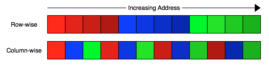
The reason you might think that writing the data column-wise would improve compression is that you might expect that e.g. the most significant bytes of a series of floats in a timeseries would be very similar to each other. By moving these similar bytes closer together you increase the chance that compression algorithms will be able to find repeating patterns in them undisturbed by the essentially random content of the LSB.
Field transposition
Analagous to the byte-level transposition described above, another thing we might try is transposition at the level of a float subcomponent. Recall that floating point numbers are divided into sign, exponent and mantissa components. For single precision floats this looks like:

Inspired by this, another thing we might try is transposing the data field-wise – i.e. serializing all the signs first, followed by all the exponents, then all the mantissas:

(Note that I’m inserting padding bits to keep multibit fields byte aligned – more on this later on.)
We might expect this transposition technique to improve compression by preventing changes in unrelated fields from causing us to be unable to spot patterns in the evolution of a certain field. A good example of where this might be useful is the sign bit: for many timeseries of interest we expect the sign bit to be uniformly 1 or 0 (i.e. all negative or all positive numbers). If we encoded the float without splitting it into fields, that that one very predictable bit is mixed in with 31 much more varied bits, which makes it much harder to spot this pattern.
Delta encoding
In delta encoding, you encode consecutive elements of a sequence not by their absolute value but rather by how much larger than they are than the previous element in the sequence. You might expect this to aid later compression of timeseries data because, although a timeseries might have an overall trend, you would expect the day-to-day variation to be essentially unchanging. For example, Vodafone’s stock price might be generally trending up from 150p at the start of the year to 200p at the end, but you expect it won’t usually change by more than 10p on any individual day within that year. Therefore, by delta-encoding the sequence you would expect to increase the probability of the sequence containing a repeated substring and hence its compressibility.
This idea can be combined with transposition, by applying the transposition to the deltas rather than the raw data to be compressed. If you do go this route, you might then apply a trick called zig-zagging (used in e.g. protocol buffers) and store your deltas such that small negative numbers are represented as small positive ints. Specifically, you might store the delta -1 as 1, 1 as 2, -2 as 3, 2 as 4 and so on. The reasoning behind this is that you expect your deltas to be both positive and negative, but certainly clustered around 0. By using zig-zagging, you tend to cause the MSB of your deltas to become 0, which then in turn leads to extremely compressible long runs of zeroes in your transposed version of those deltas.
Special cases
One particular floating point number is worth discussing: NaN. It is very common for financial timeseries to contain a few NaNs scattered throughout. For example, when a stock exchange is on holiday no official close prices will be published for the day, and this tends to be represented as a NaN in a timeseries of otherwise similar prices.
Because NaNs are both common and very dissimilar to other numbers that we might encounter, we might want to encode them with a special short representation. Specifically, I implemented a variant of the field transposition above, where the sign bit is actually stored extended to a two bit “descriptor” value with the following interpretation:
| Bit 1 | Bit 2 | Interpretation |
|---|---|---|
| 0 | 0 | Zero |
| 0 | 1 | NaN |
| 1 | 0 | Positive |
| 1 | 1 | Negative |
The mantissa and exponent are not stored if the descriptor is 0 or 1.
Note that this representation of NaNs erases the distinction between different NaN values, when in reality there are e.g. 16,777,214 distinct single precision NaNs. This technically makes this a lossy compression technique, but in practice it is rarely important to be able to distinguish between different NaN values. (The only application that I’m aware of that actually depends on the distinction between NaNs is LuaJIT.)
Methodology
In my experiments (available on Github) I tried all combinations of the following compression pipeline:
-
Field transposition: on (start by splitting each number into 3 fields) or off (treat whole floating point number as a single field)?
-
(Only if field transposition is being used.) Special cases: on or off?
-
Delta encoding: off (store raw field contents) or on (stort each field as an offset from the previous field)? When delta encoding was turned on, I additionally used zig-zagging.
-
Byte transposition: given that I have a field, should I transpose the bytes of that field? In fact, I exhaustively investigated all possible byte-aligned transpositions of each field.
-
Compressor: BZ2 or Snappy?
I denote a byte-level transposition as a list of numbers summing to the number of bytes in one data item. So for example, a transposition for 4-byte numbers which wrote all of the LSBs first, followed by the all of the next-most-significant bytes etc would be written as [1, 1, 1, 1], while one that broke each 4-byte quantity into two 16-bit chunks would be written [2, 2], and the degenerate case of no transposition would be [4]. Note that numbers occur in the list in increasing order of the significance of the bytes in the item that they manipulate.
As discussed above, in the case where a literal or mantissa wasn’t an exact multiple of 8 bits, my filters padded the field to the nearest byte boundary before sending it to the compressor. This means that the filtering process actually makes the data substantially larger (e.g. 52-bit double mantissas are padded to 56 bits, becoming 7.7% larger in the process). This not only makes the filtering code simpler, but also turns out to be essential for good compression when using Snappy, which is only able to detect byte-aligned repitition.
Without further ado, let’s look at the results.
Dense timeseries
I begin by looking at dense timeseries where NaNs do not occur. With such data, it’s clear that we won’t gain from the “special cases” encoding above, so results in this section are derived from a version of the compression code where we just use 1 bit to encode the sign.
Single-precision floats
The minimum compressed size (in bytes) achieved for each combination of parameters is as follows:
| Exponent Method | Mantissa Method | BZ2 | Snappy |
|---|---|---|---|
| Delta | Delta | 6364312 | 9067141 |
| Literal | 6283216 | 8622587 | |
| Literal | Delta | 6372444 | 9071864 |
| Literal | 6306624 | 8626114 |
(This table says that, for example, if we delta-encode the float exponents but literal-encode the mantissas, then the best tranposition scheme achieved a compressed size of 6,283,216 bytes.)
The story here is that delta encoding is strictly better than literal encoding for the exponent, but conversely literal encoding is better for the mantissa. In fact, if we look at the performance of each possible mantisas transposition, we can see that delta encoding tends to underperform in those cases where the MSB is split off into its own column, rather than being packaged up with the second-most-significant byte. This result is consistent across both BZ2 and Snappy.
| Mantissa Transposition | Mantissa Method | BZ2 | Snappy |
|---|---|---|---|
| [1, 1, 1] | Delta | 7321926 | 9199766 |
| Literal | 7226293 | 9154821 | |
| [1, 2] | Delta | 7394645 | 9317258 |
| Literal | 7824557 | 9420206 | |
| [2, 1] | Delta | 6514554 | 9099462 |
| Literal | 6283216 | 8622587 | |
| [3] | Delta | 6364312 | 9067141 |
| Literal | 6753718 | 9475316 |
The other interesting feature of these results is that transposition tends to hurt BZ2 compression ratios. It always makes things worse with delta encoding, but even with literal encoding only one particular transposition ([2, 1]) actually strongly improves a BZ2 result. Things are a bit different for Snappy: although once again delta is always worse with transposition enabled, transpostion always aids Snappy in the literal case – though once again the effect is strongest with [2, 1] transposition.
The strong showing for [2, 1] transposition suggests to me that the lower-order bits of the mantissa are more correlated with each other than they are with the MSB. This sort of makes sense, since due to the fact that equities trade with a fixed tick size prices will actually be quantised into a relatively small number of values. This will tend to cause the lower order bits of the mantissa to become correlated.
Finally, we can ask what would happen if we didn’t make the mantissa/exponent distinction at all and instead just packed those two fields together:
| Method | BZ2 | Snappy |
|---|---|---|
| Delta | 6254386 | 8847839 |
| Literal | 6366714 | 8497983 |
These numbers don’t show any clear preference for either of the two approaches. For BZ2, delta performance is improved by not doing the splitting, at the cost of larger outputs when using the delta method, while for Snappy we have the opposite: literal performance is improved while delta performance is harmed. What is true is that the best case, the compressed sizes we observe here are better than the best achievable size in the no-split case.
In some ways it is quite surprising that delta encoding ever beats literal encoding in this scenario, because it’s not clear that the deltas we compute here are actually meaningful and hence likely to generally be small.
We can also analyse the best available transpositions in this case. Considering BZ2 first:
| BZ2 Rank | Delta Transposition | Size | Literal Transposition | Size |
|---|---|---|---|---|
| 1 | [4] | 6254386 | [2, 2] | 6366714 |
| 2 | [3, 1] | 6260446 | [2, 1, 1] | 6438215 |
| 3 | [2, 2] | 6395954 | [3, 1] | 7033810 |
| 4 | [2, 1, 1] | 6402354 | [4] | 7109668 |
| 5 | [1, 1, 1, 1] | 7136612 | [1, 1, 1, 1] | 7327437 |
| 6 | [1, 2, 1] | 7227282 | [1, 1, 2] | 7405128 |
| 7 | [1, 1, 2] | 7285350 | [1, 2, 1] | 8039403 |
| 8 | [1, 3] | 7337277 | [1, 3] | 8386647 |
Just as above, delta encoding does best when transposition at all is used, and generally gets worse as the transposition gets more and more “fragmented”. On the other hand, literal encoding does well with transpositions that tend to keep together the first two bytes (i.e. the exponent + the leading bits of the mantissa).
Now let’s look at the performance of the unsplit data when compressed with Snappy:
| Snappy Rank | Delta Transposition | Size | Literal Transposition | Size |
|---|---|---|---|---|
| 1 | [3, 1] | 8847839 | [2, 1, 1] | 8497983 |
| 2 | [2, 1, 1] | 8883392 | [1, 1, 1, 1] | 9033135 |
| 3 | [1, 1, 1, 1] | 8979988 | [1, 2, 1] | 9311863 |
| 4 | [1, 2, 1] | 9093582 | [3, 1] | 9404027 |
| 5 | [2, 2] | 9650796 | [2, 2] | 10107042 |
| 6 | [4] | 9659888 | [1, 1, 2] | 10842190 |
| 7 | [1, 1, 2] | 9847987 | [4] | 10942085 |
| 8 | [1, 3] | 10524215 | [1, 3] | 11722159 |
The Snappy results are very different from the BZ2 case. Here, the same sort of transpositions tend to do well with both the literal and delta methods. The kinds of transpositions that are successful are those that keep together the exponent and the leading bits of the mantissa, though even fully-dispersed transpositions like [1, 1, 1, 1] put in a strong showing.
That’s a lot of data, but what’s the bottom line? For Snappy, splitting the floats into mantisas and exponent before processing does seem to have slightly more consistently small outputs than working with unsplit data. The BZ2 situation is less clear but only because the exact choice doesn’t seem to make a ton of difference. Therefore, my recommendation for single-precision floats is to delta-encode exponents, and to use literal encoding for mantissas with [2, 1] transposition.
Double-precision floats
While there were only 4 different transpositions for single-precision floats, there are 2 ways to transpose a double-precision exponent, and 64 ways to transpose the mantissa. This makes the parameter search for double precision considerably more computationally expensive. The results are:
| Exponent Method | Mantissa Method | BZ2 | Snappy |
|---|---|---|---|
| Delta | Delta | 6485895 | 12463583 |
| Literal | 6500390 | 10437550 | |
| Literal | Delta | 6456152 | 12469132 |
| Literal | 6475579 | 10439869 |
These results show interesting differences between BZ2 and Snappy. For BZ2 there is not much in it, but it’s consistently always better to literal-encode the exponent and delta-encode the mantissa. For Snappy, things are exactly the other way around: delta-encoding the exponent and literal-encoding the mantissa is optimal.
The choice of exponent transposition scheme has the following effect:
| Exponent Transposition | Exponent Method | BZ2 | Snappy |
|---|---|---|---|
| [1, 1] | Delta | 6485895 | 10437550 |
| Literal | 6492837 | 10439869 | |
| [2] | Delta | 6496032 | 10560467 |
| Literal | 6456152 | 10564737 |
It’s not clear, but [1, 1] transposition might be optimal. Bear in mind that double exponents are only 11 bits long, so the lower 5 bits of the LSB being encoded here will always be 0. Using [1, 1] transposition might better help the compressor get a handle on this pattern.
When looking at the best mantissa transpositions, there are so many possible transpositions that we’ll consider BZ2 and Snappy one by one, examining just the top 10 transposition choices for each. BZ2 first:
| BZ2 Rank | Delta Mantissa Transposition | Size | Literal Mantissa Transposition | Size |
|---|---|---|---|---|
| 1 | [7] | 6456152 | [6, 1] | 6475579 |
| 2 | [6, 1] | 6498686 | [1, 5, 1] | 6495555 |
| 3 | [4, 3] | 6962167 | [2, 4, 1] | 6510416 |
| 4 | [4, 2, 1] | 6994270 | [1, 1, 4, 1] | 6510416 |
| 5 | [1, 6] | 7040401 | [3, 3, 1] | 6692613 |
| 6 | [3, 4] | 7054835 | [2, 1, 3, 1] | 6692613 |
| 7 | [1, 5, 1] | 7092230 | [1, 1, 1, 3, 1] | 6692613 |
| 8 | [2, 5] | 7108000 | [1, 2, 3, 1] | 6692613 |
| 9 | [2, 4, 1] | 7176760 | [1, 6] | 6926231 |
| 10 | [3, 3, 1] | 7210100 | [7] | 6931475 |
We can see that literal encoding tends to beat delta encoding, though the very best size was in fact achieved via a simple untransposed delta representation. In both the literal and the delta case, the encodings that do well tend to keep the middle 5 bytes of the mantissa grouped together, which is support for our idea that these bytes tend to be highly correlated, with most of the information being encoded in the MSB.
Turning to Snappy:
| Snappy Rank | Delta Mantissa Transposition | Size | Literal Mantissa Transposition | Size |
|---|---|---|---|---|
| 1 | [5, 1, 1] | 12463583 | [3, 2, 1, 1] | 10437550 |
| 2 | [1, 3, 2, 1] | 12678887 | [1, 1, 1, 2, 1, 1] | 10437550 |
| 3 | [6, 1] | 12737838 | [1, 2, 2, 1, 1] | 10437550 |
| 4 | [4, 2, 1] | 12749067 | [2, 1, 2, 1, 1] | 10437550 |
| 5 | [7] | 12766804 | [1, 1, 1, 1, 1, 1, 1] | 10598739 |
| 6 | [1, 3, 1, 1, 1] | 12820360 | [2, 1, 1, 1, 1, 1] | 10598739 |
| 7 | [3, 1, 2, 1] | 12824154 | [3, 1, 1, 1, 1] | 10598739 |
| 8 | [4, 1, 1, 1] | 12890981 | [1, 2, 1, 1, 1, 1] | 10598739 |
| 9 | [3, 3, 1] | 12915900 | [1, 1, 1, 1, 2, 1] | 10715444 |
| 10 | [3, 1, 1, 1, 1] | 12946767 | [3, 1, 2, 1] | 10715444 |
The Snappy results are strikingly different from the BZ2 ones. In this case, just like BZ2, literal encoding tends to beat delta encoding, but the difference is much more pronounced than the BZ2 case. Furthermore, the kinds of transpositions that minimize the size of the literal encoded data here are very different from the transpositions that were successful with BZ2: in that case we wanted to keep the middle bytes together, while here the scheme [1, 1, 1, 1, 1, 1, 1] where every byte has it’s own column is not far from optimal.
And now considering results for the case where we do not split the floating point number into mantissa/exponent components:
| Method | BZ2 | Snappy |
|---|---|---|
| Delta | 6401147 | 11835533 |
| Literal | 6326562 | 9985079 |
These results show a clear preference for literal encoding, which is definitiely what we expect, given that delta encoding is not obviously meaningful for a unsplit number. We also see results that are universally better than those for split case: it seems that splitting the number into fields is actually a fairly large pessimisation! This is probably caused by the internal fragmentation implied by our byte-alignment of the data, which is a much greater penalty for doubles than it was for singles. It would be interesting to repeat the experiment without byte-alignment.
We can examine which transposition schemes do best in the unsplit case. BZ2 first:
| BZ2 Rank | Delta Transposition | Size | Literal Transposition | Size |
|---|---|---|---|---|
| 1 | [8] | 6401147 | [6, 2] | 6326562 |
| 2 | [7, 1] | 6407935 | [1, 5, 2] | 6351132 |
| 3 | [6, 2] | 6419062 | [2, 4, 2] | 6360533 |
| 4 | [6, 1, 1] | 6440333 | [1, 1, 4, 2] | 6360533 |
| 5 | [4, 3, 1] | 6834375 | [3, 3, 2] | 6562859 |
| 6 | [4, 4] | 6866167 | [1, 2, 3, 2] | 6562859 |
| 7 | [4, 2, 1, 1] | 6903123 | [2, 1, 3, 2] | 6562859 |
| 8 | [4, 2, 2] | 6903322 | [1, 1, 1, 3, 2] | 6562859 |
| 9 | [1, 7] | 6979216 | [6, 1, 1] | 6598104 |
| 10 | [1, 6, 1] | 6983998 | [1, 5, 1, 1] | 6621003 |
Recall that double precision floating point numbers have 11 bits of exponent and 52 bits of mantissa. We can actually see that showing up in the literal results above: the transpositions that do best are those that either pack together the exponent and the first bits of the mantissa, or have a seperate column for just the exponent information (e.g. [1, 5, 2] or [2, 4, 2]).
And Snappy:
| Snappy Rank | Delta Transposition | Size | Literal Transposition | Size |
|---|---|---|---|---|
| 1 | [5, 1, 1, 1] | 11835533 | [1, 1, 1, 2, 1, 1, 1] | 9985079 |
| 2 | [1, 3, 2, 1, 1] | 12137223 | [2, 1, 2, 1, 1, 1] | 9985079 |
| 3 | [6, 1, 1] | 12224432 | [3, 2, 1, 1, 1] | 9985079 |
| 4 | [4, 2, 1, 1] | 12253670 | [1, 2, 2, 1, 1, 1] | 9985079 |
| 5 | [1, 3, 1, 1, 1, 1] | 12280165 | [1, 1, 1, 1, 1, 1, 1, 1] | 10232996 |
| 6 | [3, 1, 2, 1, 1] | 12281694 | [2, 1, 1, 1, 1, 1, 1] | 10232996 |
| 7 | [5, 1, 2] | 12338551 | [1, 2, 1, 1, 1, 1, 1] | 10232996 |
| 8 | [4, 1, 1, 1, 1] | 12399017 | [3, 1, 1, 1, 1, 1] | 10232996 |
| 9 | [3, 1, 1, 1, 1, 1] | 12409691 | [1, 1, 1, 1, 2, 1, 1] | 10343471 |
| 10 | [2, 2, 2, 1, 1] | 12434147 | [2, 1, 1, 2, 1, 1] | 10343471 |
Here we see the same pattern as we did above: Snappy seems to prefer “more transposed” transpositions than BZ2 does, and we even see a strong showing for the maximal split [1, 1, 1, 1, 1, 1, 1, 1].
To summarize: for doubles, it seems that regardless of which compressor you use, you are better off not splitting into mantissa/exponent portions, and just literal encoding the whole thing. If using Snappy, [1, 1, 1, 1, 1, 1, 1, 1] transposition seems to be the way to go, but the situation is less clear with BZ2: [6, 2] did well in our tests but it wasn’t a runaway winner.
If for some reason you did want to use splitting, if you are also going to use BZ2, then [6, 1] literal encoding for the mantissas and literal encoding for the exponents seems like a sensible choice. If you are a Snappy user, then I would suggest that a principled choice would be to use [1, 1, 1, 1, 1, 1, 1] literal encoding for the mantissas and likewise [1, 1] literal encoding for the exponent.
Sparse timeseries
Let’s now look at the sparse timeseries case, where many of the values in the timeseries are NaN. In this case, we’re interested in evaluating how useful the “special case” optimization above is in improving compression ratios.
To evaluate this, I replaced a fraction of numbers in my test dataset with NaNs and looked at the best possible size result for a few such fractions. The compressed size in each case is:
| No Split | Split w/ Special Cases | Split wout/ Special Cases | |
|---|---|---|---|
| 0.00 | 9985079 | 10445497 | 10437550 |
| 0.10 | 10819117 | 9909251 | 11501526 |
| 0.50 | 8848393 | 6238097 | 10255811 |
| 0.75 | 5732076 | 3628543 | 7218287 |

Note that for convenience here the only compressor I tested was Snappy – i.e. BZ2 was not tested. I also didn’t implement special cases in the no-split case, because an artifact of my implementation is that the special-casing is done at the same time as the float is split into its three component fields (sign, mantissa, exponent).
As we introduce small numbers of NaNs to the data, both the nosplit and non-special-cased data get larger. This is expected, because we’re replacing predictable timeseries values at random with totally dissimilar values and hence adding entropy. The special-cased split shrinks because this increasing entropy is compensated for by the very short codes we have chosen for NaNs (for which we do pay a very small penalty in the NaNless case). At very high numbers of NaNs, the compressed data for all methods shrinks as NaNs become the rule rather than the exception.
High numbers of NaNs (10% plus) is probably a realistic fraction for real world financial data, so it definitely does seem like implementing special cases is worthwhile. The improvement would probably be considerably less if we looked at BZ2-based results, though.
Closing thoughts
One general observation is that delta encoding is very rarely the best choice, and when it is the best, the gains are usually marginal when compared to literal encoding. This is interesting because Fabian Giesen came to exactly the same conclusion (that delta encoding is redundant when you can do transposition) in the excellent presentation that I linked to earlier.
By applying these techniques to the dataset I was dealing with at work, I was able to get a nice compression ratio on the order of 10%-20% over and above that I could achieve with naive use of Snappy, so I consider the work a success, but don’t intend to do any more research in the area. However, there are definitely more experiments that could be done in this vein. In particular, interesting questions are:
- How robust are the findings of this post when applied to other datasets?
- What if we don’t byte-align everything i.e. remove some of the useless padding bits? Does that improve the BZ2 case? (My prelimiary experiments showed that it made Snappy considerably worse.)
- Why exactly are the results for BZ2 and Snappy so different? Presumably it relates to the lack of an entropy encoder is Snappy, but it is not totally clear to me how this leads to the results above.